|
Abstract
Canny's edge detector assumes a Gaussian filter as its enhancer at the enhancement
stage of the algorithm. While suitable for smoothing noises, a Gaussian filter can
not adapt to varying illumination seen in most real-world images, consequently rendering
a sub-optimal enhancement for edge detection. In this paper, I present a novel approach,
the "membrane-difference" method based on Cellular Neural Network's falling membrane
filter, to achieve space-variant feature enhancement that improves Canny's edge
detector. With such enhancement, experiments show that even with simple-minded,
lazy use of Matlab 5.2' Canny edge detector with default parameters, one can obtain
improved edge maps that one might otherwise get only by many trial-and-errors with
Canny's three parameters.
- Introduction
Gaussian filters are not the best image enhancers. While adept at noise
smoothing, they cannot adapt to variations in image illumination. When used in feature
enhancement for images under space-varying illumination, they perform less well
because of this fundamental limit (they cannot help expose features "hidden" in
the scene due to uneven illumination in the image.)
The ever popular Canny's edge detector in its standard form (as presented
in class and in the textbook [1])
assumes, however, a Gaussian filter as its enhancer at the first stage of the algorithm.
Consequently, one would expect that objects in images subject to uneven illumination
are likely to be poor targets for Canny's, simply because the space-invariant, Gaussian
filter is ill-suited to enhance features in such objects. In such cases (in fact,
most real-world images are subject to space varying illumination to certain extent),
Canny's renders sub-optimal enhancements that act as subpar inputs to subsequent
stages. Tweaking the three magic numbers (sigma, low and high) of the algorithm,
though helpful, seems ad hoc in these situations. If the enhancement stage uses
an adaptive, space-variant filter, perhaps one can tweak less frequently the three
parameters while still obtain good results across a wider set of images.
In this project, I propose a new method that uses Cellular Neural Network's
falling membrane filter [2],
which I will call the "membrane-difference" method, to help enhancing features at
the first stage of Canny's algorithm. I will show that with such method, a no-brainer
use of Matlab 5.2's Canny edge detector will result in improved edge maps that might
otherwise be obtained only by many trial-and-errors with Canny's parameters.
Invented by Chua and Yang in '88, Cellular Neural Network (CNN) presents
an intriguingly new paradigm for computing and is inherently well-suited for image
processing applications. Because of its drastically different computation architecture
and theory (from those of traditional digital computers), lest the paper becomes
unnecessarily lengthy, I will not present an introduction to CNN here. Instead,
I refer interested readers to the bibliography section of Crounse's paper [2]
for definitive and many interesting papers on CNN (particularly, Chua and Yang's
papers [3]-[4] on the
theory and applications of CNN are worth reading.) Though without full (or any)
understanding of the makings of a CNN algorithm, I believe that, and will strive
to illustrate my method so that, any reader familiar with basic image processing
and Canny's edge detector can easily digest the discussion in this paper.
- The Method
In his thesis paper [2],
Crounse mentions a CNN falling membrane filter to effectively enhance image contrast
in microscopy applications. He creates the membrane filter to obtain a space-variant
estimate of image illumination, which is then subtracted from the original image
in the contrast domain to obtain the illumination- (shadow-) removed, contrast-enhanced
version of the image. While suitable to his particular application at hand, such
illumination-removal method is less so for detecting edges in images. The main reason
is that such process over-amplifies noises in the images (especially in the dark
regions), effectively perturbing the original image a bit too much to be desirable
in the edge detection domain.
The space-variant structure of the membrane, however, is intriguing.
My proposed membrane-difference method, in fact, takes advantage of the space-varying
difference between the membrane and the image surface to enhance image features
subject to uneven illumination.
2.1 The Falling Membrane
Imagine dropping a thin membrane (through a viscous, momentumless medium)
onto an image's intensity surface under the effect of gravity in the downward direction.
As time goes by, only the local maxima of the image surface counteract the gravity's
effect, preventing the membrane from falling completely onto the bottom of the image
surface. Consequently, as this process converges toward equilibrium, the shape of
the membrane approximates the image surface while sags into valleys. To visually
illustrate this process, let's take, as an example, a synthetic image composed of
step edges as shown in Figure 1. Figure 2 shows a 1D intensity surface along one
row of the image, "u", and the shape of the resultant membrane, "membrane" (produced
by my membrane.m with default parameters (I=-1.0 and tf=10). Please see "Implementation
Note" for how this implementation of falling membrane differs slightly from the
one shown on p. 205 of Crounse's paper [2],
and why this is better-suited for edge enhancement.)

|
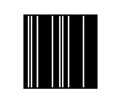
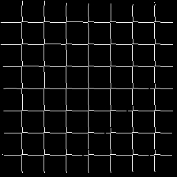
Figure 1. A 50x50 synthetic image used for illustrating the concept
of the falling membrane idea and my proposed method (note the image is scaled up
to be 100x100 for ease of viewing.)
|
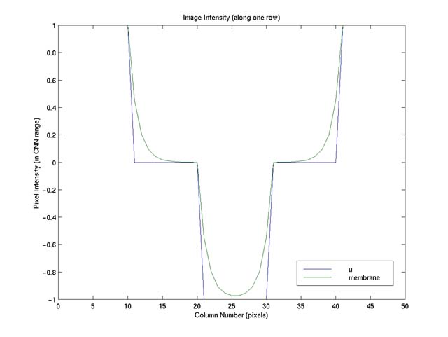
Figure 2. The plot of the image intensity surface ("u") and the membrane
("membrane," the fine dash line), produced by membrane.m using default parameters,
along one row of the image shown in Figure 1. This plot (and similar ones below)
is shown in CNN's native pixel intensity range of [-1, 1]: -1 corresponds to darkest
pixels; 1 the brightest.
2.2 The Space-Variant Feature Enhancement
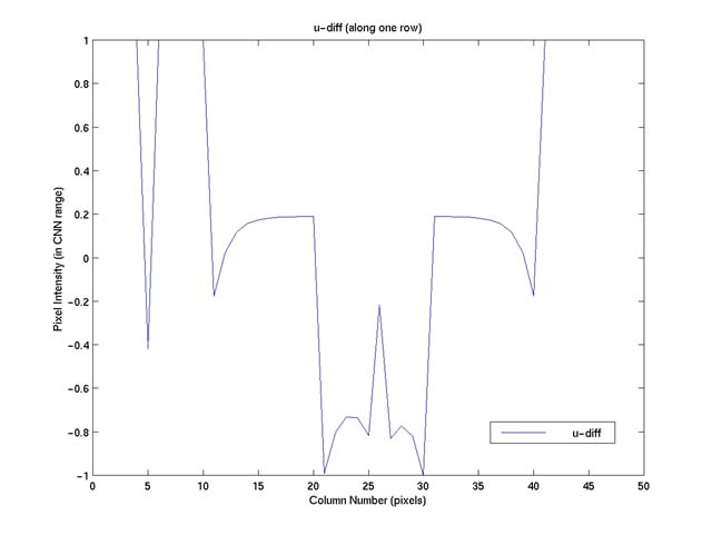
If we now subtract the difference, "diff," between the membrane and
the image surface (Figure 3) from the image, we get the results as shown in Figure
4.
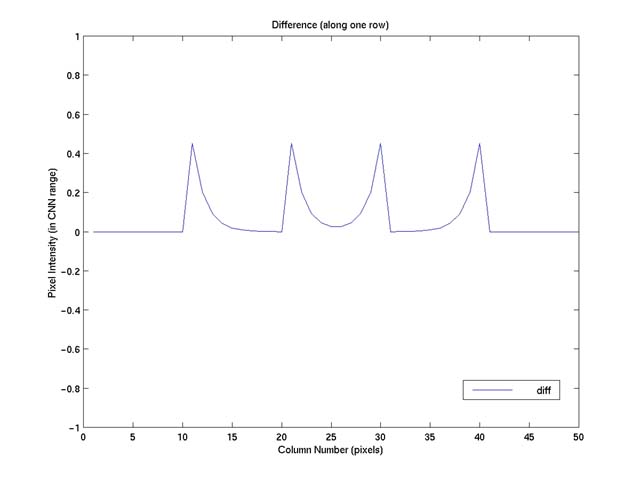
Figure 3. The difference, "diff", between the membrane and the image
surface. "diff" equals to one plus the direct output of CNN, the "output" in my
membrane.m and "y" in p. 202 of Crounse's paper [2].
In my actual implementation, I directly use "u"-"output" for later computation since
the vertical offset of one doesn't matter for internal image operations.
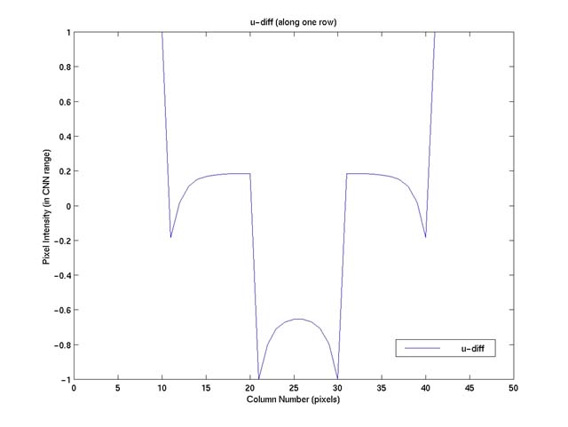
Figure 4. The result of "u" - "diff," scaled back to CNN's pixel intensity
range.
As we can see, this simple, interesting operation in effect enhances
the edges (i.e. the regions between peaks followed immediately by valleys or vice
versa), brightens the flat, dark regions a bit, while leaves the flat, bright regions
(the high plateau) of the image surface unchanged (in intensity). Figure 5 shows
the effect of such operation on a real image (because the original image is too
small to comfortably see detailed edges, I decide not to show the enhanced edge
map and only use it to illustrate the resultant enhancement on the original image.)
 (a) (a)
 (b) (b)
Figure 5. (a) The original image. (b) The enhanced image ("u"-"diff,"
both produced by membrane.m with default parameters).
In a real image, though, noises are likely to exist in both the bright
and dark regions of the image surface. This operation, consequently, will amplify
the noises a bit in both regions ("a bit," assuming noises and their surrounding
regions differ relatively "little" in intensity values -- relative to the difference
one usually sees for edges). This means a Gaussian filter at this point is desirable
before performing edge detection. Therefore, if we actually follow this membrane-difference
operation by the standard Canny's edge enhancement method without any change (i.e.
the Gaussian filter), we obtain a space-variant, noise-smoothed feature enhancement
at the enhancement stage of Canny's algorithm. Figure 6 illustrates this process
visually (on a synthetic image similar to Figure 1).
 (a)
(a)
 (b)
(b)
 (c)
(c)
 (d)
(d)
 (e)
(e)
 (f)
(f)
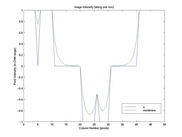
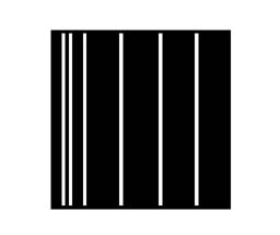
Figure 6. (a) An image very similar to Figure 1; only this time, I add
a valley, an edge, in the bright region, and a noise (since its magnitude is small
relative to other "edges") in the dark region. (b) Plot of the image surface, "u,"
and the membrane (using membrane.m with default parameters) along one row of the
image. (c) The result of "u"-"diff," scaled back the CNN's pixel intensity range.
(d) The edge map produced by Canny's on "u"-"diff" without Gaussian-smoothing (by
running cannyNoGauss.m) -- both the edge and the noise are detected. (For ease of
viewing, this edge map, as well as (e) and (f) is scaled up to be 100x100 -- because
of unprofessional scaling and cropping, sizes of the black edge maps are a bit different.)
(e) The final edge map produced by Matlab 5.2's Canny edge detector with default
parameters. One can see that now Canny's detects the edge in the bright region,
while ignores the noise in the dark region. (f) The original edge map produced by
Canny's. One can see that it includes the edge in the bright region, while ignores
the noise in the dark region as well, thanks to Gaussian blurring. By comparing
(e) and (f), one can see that the membrane-difference method also enhances the image,
helping Canny's so that the detected edges are now straight.
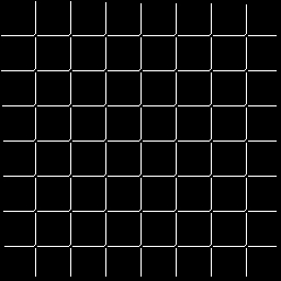
Figure 7 shows how the method (with default parameters) improves the
performance of Canny's edge detector on a popular, synthetic checker-pattern image.
While it is a bit hard to visually detect the subtle improved difference between
the original and enhanced images, one can easily see that the detected edges are
better than the original ones using Canny's. (Unless explicitly mentioned, I use
default parameters when comparing performance between original Canny's and my method,
i.e. sigma=1, low and high thresholds automatically selected. For all comparisons,
to be fair to both algorithms, I apply the same set of Canny's parameters.)
 (a)
(a)
 (c)
(c)
 (b)
(b)
 (d)
(d)
Figure 7. (a) The checker-pattern image. (b) The edge map found by Matlab
5.2's Canny edge detector with default parameters. (c) The enhanced output image
by the membrane-difference method. (d) The improved edge map produced by Canny's
(with default parameters) on (c).
2.2 Implementation Note
This version of the falling membrane filter is slightly different from
the one shown in p. 205 of Crounse's paper [2].
Specifically, this version uses, for both templates, a center element of -4 and
0.5 for the others in the 3x3 neighborhood. This is so that the gravity effect is
"height-dependent," i.e. in deep intensity valleys, the membrane will fall (sag)
much more than the one produced by the original templates. As mentioned in Figures
8.3 and 8.4 (on pp. 204-205) of his paper, the original templates produce a membrane
that sags only slightly into valleys -- while desirable in that context, this is
less so for the membrane-difference method used for detecting edges, since taking
the difference between "u" and "diff" will now brighten the dark regions too much
and over-amplify the noises in both bright and dark regions. Such effect, to certain
extent, is desirable in some special situations. Yet in such cases, one can also
achieve similar effect using the modified version by adjusting the final time parameter
(i.e. the time we allow the membrane to fall through the surface and converge to
equilibrium). I will illustrate this special situation in the "Shadow" image in
the next section.
Another difference lies in the default parameter used for gravity.
This version uses -1.0 instead of -0.05 since it behaves better in general with
the modified templates (one simply works out the CNN equations to decide on a good
default value.) Furthermore, a stronger gravity also shortens the time required
for convergence, much more so than that typically needed in the original version
(so one doesn't need to wait that long before obtaining a satisfactory membrane).
This time-saving is especially nice given that the Matlab CNN simulator already
runs very slowly on large images (this is a software simulator for an analogic neural
network architecture, after all.)
With this modified version, I have found that running the CNN simulator
for ten time steps suffices for most images in general. Therefore, in the attached
code, the default final time (tf) is 10, while the default gravity (I) is -1.0.
Unless otherwise mentioned, these are also the parameters used for sample experiments
presented in this paper.
- Experiments and Further Analysis with Real, Sample Images
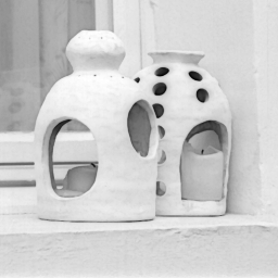
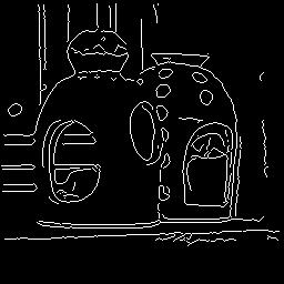
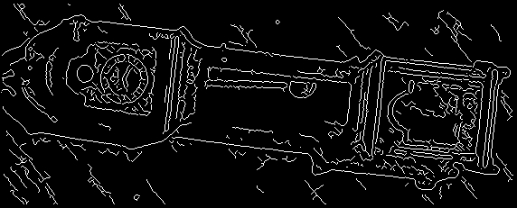
First, I apply the membrane-difference method to the "Lamp" picture
shown in Figure 8. One can see that this method helps pick out even edges of the
lamp reflection in the background window.
![]() (a)
(a)
 (c)
(c)
 (b)
(b)
 (d)
(d)
Figure 8. Lamp image: (a) The original. (b) The detected edge map using
Canny's. (c) The enhance image. (d) The enhanced edge map.
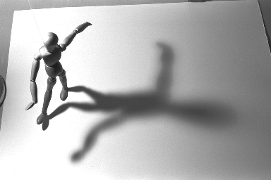
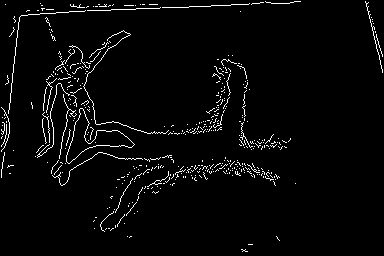
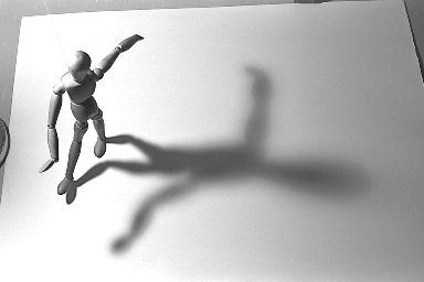
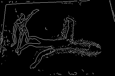
Figure 9 shows the result when by applying the method to the "Shadow"
image that contains very smoothly-varying shadow and different degrees of illumination
in the image. Although one does see an improved edge map (e.g. edges around the
sheet are picked up more nicely and appear more continuous; the circle on the wooden
doll's head is now closed; fewer noises appear in general), one could argue that
the enhancement leaves something to be desired. Specifically, fewer shadow's edges
remain as a result of the membrane-difference method, i.e. edges around the upper
half of the shadow disappear now. One can find the reason behind this reduction
by looking at the enhanced image. Because the dark regions of the shadow head are
now brightened a bit too much (relative to its immediate surroundings), edges of
the shadow head lose a bit of their original degrees of contrast. Although the membrane-difference
method is supposed to increase the contrast around edges, because of the slowly-varying
intensity from the dark core of the shadow head to its less dark surroundings, the
membrane-difference actually loses its keen ability a bit to strengthen edges in
this region -- with default parameters, that is.
 (a)
(a)
|
 (c)
(c)
|
 (b)
(b)
|
 (d)
(d)
|
|
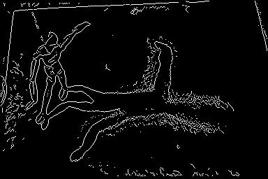
Figure 9. Shadow image: (a) The original. (b) Edge map found by Canny's.
(c) The enhanced image. (d) The enhanced edge map.
|
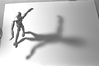
To remedy such defect, i.e. when one would like the membrane-difference
method to strengthen edges in the dark regions better than usual (in this case,
extracting edges from the shadow better), one can decide not to use the default
parameters of the membrane-difference method. By running the CNN simulator, say,
just for one timestep instead of ten, we know that the membrane is still high above
the valleys in such short amount of time, as it hasn't converged well to its final
shape. The resultant "diff" in this case will then have large values for dark regions
in the image; effectively, "u"-"diff" will enable the shadow head to lose less of
its intensity. Furthermore, to strengthen the edges (at a slight cost of amplifying
noises a bit more), one can increase the gravity so that in a short amount of time,
relatively shallower valleys (e.g. between the shadow head and its immediate surroundings)
can now be deepened a bit more . With these two improvements in mind, Figure 10
shows the newly improved image by using gravity value of -1.7 and tf value of 1.
One can see that the shadow edges are now much better, while the improved edges
found in Figure 9(d) remain there in general (although the circle in the doll's
head and the suspending string
, for instance, lose a bit of the continuity as shown in Figure 9(d).)
 (a)
(a)
 (b)
(b)
Figure 10. (a) The new enhanced image using I=-1.7 with tf=1. (b) The
new edge map.
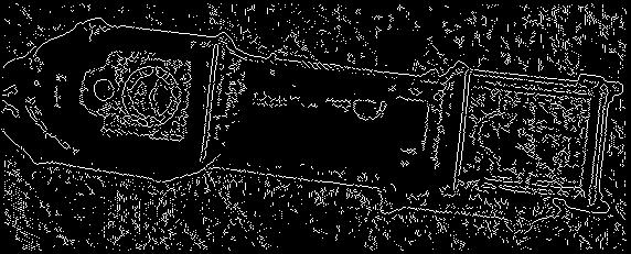
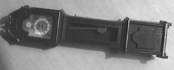
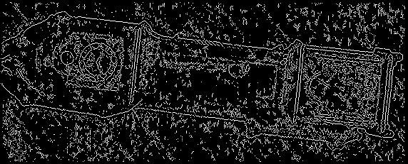
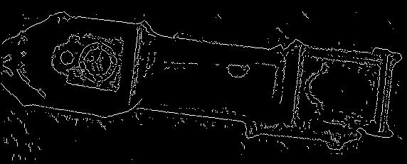
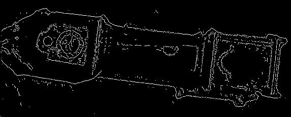
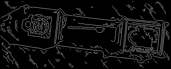
Finally, just to take on a challenge, I apply the method, using I=-2
and tf=1 (for reasons similar to those for "Shadow"), to the "Clock" image grabbed
from the web (Figure 11(a)), whose supposedly fine textures in most regions appear
very rough probably because the inadequate gif format is used to save the original
image, or perhaps because it is intentionally made up to be so (?) (to be consistent
with all other image formats presented here, I convert it to jpeg for web-viewing
though.) Most regions in this image, therefore, contain many sharp noises at this
point. Consequently, while applying the membrane-difference operation to such image
still improves the edge map (Figure 11(d)), it also amplifies noises (in this case,
in the dark regions because it tries to accentuate edges here -- how
I wish for a footnote equivalent here) to a degree that can't be quite
compensated for by Gaussian smoothing (with default sigma=1) -- hence a minor weakness
of the method ("minor" since one can claim that this type of image violates the
noise assumption a bit too much (see Section 2.2)
). To reduce noises, one can, for example, increase the Gaussian sigma to be 2,
instead of the default 1 (at the cost of losing more features). Figure 11(f) shows
such result, which is essentially the same as that from standard Canny's with sigma
2 (Figure 11(e)) -- notice that many, originally enhanced edges have also been blurred
away because Canny's finds them mostly to be short edges to begin with. For such
unpleasantly noisy image, one can try bilateral filtering [5]
before Canny's edge detection to help reduce noises while preserve the enhanced
edges: sigmaR=30 and sigmaD=1 turn out to work well for this purpose -- sigmaD=1
for Canny's, by default, has another Gaussian smoothing with sigma=1 so one probably
doesn't want sigmaD to be large; sigmaR is some experimental guess. With bilateral
filtering used in this type of image, one can now easily see the improvement in
the edge map.
 (a)
(a)
 (b)
(b)
 (c)
(c)
 (d)
(d)
 (e)
(e)
 (f)
(f)
 (g)
(g)
 (h)
(h)
Figure 11. Clock image: (a) The original image. (b) Canny's output.
(c) The enhanced image. (d) The supposedly enhanced edge map. Edges of the pendulum
and its containing rectangle, for instance, are clearer. Yet because of the great
amount of sharp noises in the original image, the final edge map contains many noises.
(e) The original Canny's output with Gaussian sigma = 2. (f) The enhanced map with
Gaussian sigma = 2. One can see that (e) and (f) are basically the same at this
point -- Gaussian with sigma 2 is enough to get rid of noises slightly over-emphasized
by the membrane-difference method. (g) Bilateral filtered (sigmaR=30, sigmaD=1)
followed by Canny's. (h) Operation sequence similar to (g), only this time preceded
by the membrane-difference method. One can now obtain a much less noisy map with
enhanced edges.
- Recommendation for Future Work
As illustrated in examples above, tuning the gravity (I), and the time
we allow membrane to converge to equilibrium (tf), can result in different performance
of the membrane-difference method. Depending on the particular image, such effects
may be desirable. There are, however, some other areas of this method that one can
explore to potentially improve the performance of the method. For instance, one
can
- Change the structure of membrane (by changing the CNN templates) so that the membrane
sags less into valleys (i.e. potential edge features). This way, the difference
operation between "u" and "diff" could enhance many edges more, at a slight cost
of amplifying the noises -- but some compromise can probably be reached. For instance,
a good combination of the original templates, larger gravity (than -0.05) and longer
tf (certainly more than 10, since the original version takes more time to converge)
can perhaps achieve a better control of the membrane-difference method to enhance
edges.
- Explore other ways to combine different values of tf and I. Although the default
parameters seem to work well for general images, one also notices that in certain
situations, larger gravity and very short tf (e.g. 1) can help. Some combination
in between may turn out to help other types of images a bit more.
- Conclusion
Taking the difference between a reasonable image and its membrane achieves space-variant
feature(edge) enhancement without over-amplifying noises. Through analysis and sample
experiments, this paper has shown that the membrane-difference method, based on
Cellular Neural Network's computation paradigm, improves Canny's edge detector at
the enhancement stage of the algorithm, rendering enhanced edge maps that may be
hard to obtain by tweaking Canny's three magic numbers alone.
Sample experiments have also shown how image-dependent adjustments on the gravity
and tf parameters appeal to intuitive, analytical, rather than arbitrary sense.
Exploring different membrane structures, and finer analysis on how different combinations
of the parameters can help other types of images, however, are desirable and should
improve robustness of the membrane-difference method.
Part of my original motivation for using CNN's method is to expose
such intriguing, promising paradigm to the vision community; the other part is that
I see interesting, potential uses of the falling membrane structure to help different
image/vision applications.
With the work presented here, I hope that I have done justice to my original motivation,
and that any interested reader will also find CNN as promising and interesting as
I do.
- Acknowledgment
Many thanks to Kenneth
R. Crounse of Berkeley for his help in providing me with the CNN Matlab
simulator, and in explaining, thus helping me appreciate, the subtlety involved
in his falling membrane design.
Also thanks to Carlo Tomasi,
the professor here, for providing me with bilateral filtering source code. Too bad
I don't have enough time to do a full comparison between my membrane-difference
method and bilateral filtering -- now that will be a cool project for next
year's students :)
- Source Code
Here is the
directory containing all the relevant Matlab files used for producing results
shown in this report.
|